How Do You Optimize an ETL Process for Speed and Cost?

This guide will give you ETL process optimization tips and a 5-step blueprint to fix pipeline lag.

I remember years ago when one morning I arrived at the office and my ETL pipeline was still running. It should be done by 6:00 AM, but it’s not. Checking the runtime history proved that over time, data grew and I’m doing a full load. Not good. If the target has been a cloud data warehouse like Snowflake, it would have blown up the bills. If you have a similar experience, it’s time for an ETL process optimization.

In this guide, I will enumerate the problems and share examples and strategies to fix performance problems.

Quick disclosure: We are the team behind Skyvia, a cloud data integration and management platform. We built it to solve these exact efficiency challenges using automated, low-code pushdown architecture. While we are naturally proud of our platform, this guide is designed to be an objective, highly technical deep dive into ETL optimization principles—regardless of whether you build custom Python pipelines or use another integration tool.

How Did We Bench-Test and Measure These ETL Optimization Techniques?

Let me tell you about our source and target systems for these ETL process optimization tests.

Source Systems

We’re going to use a PostgreSQL database hosted in Neon. As you can see below, we have 50,000 orders and a million order items:

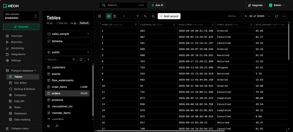
Now, don’t get too focused on a million-row dataset. We will use that full dataset as applicable to the test we will perform. There will be tests that will use fewer rows, as I don’t want to blow up my own data warehouse bills.

Also, we need a 10,000-row CSV file to demonstrate ways that will make the ETL process slow and another that will make it really fast. It’s a customer file as seen below:

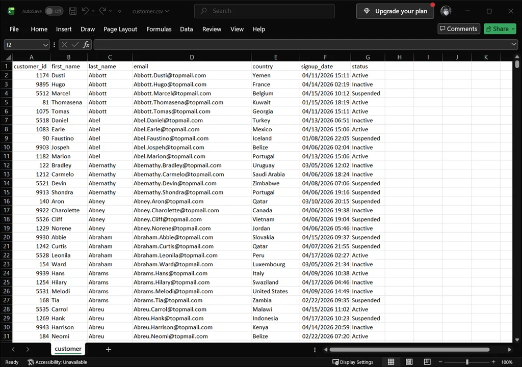
The names and email addresses are fictional and for test purposes only.

For techniques needing API rate limit control, HubSpot is our choice.

Target Warehouses

We’re going to use a dataset in BigQuery. We need counterparts for the customers and orders. You can see them below:

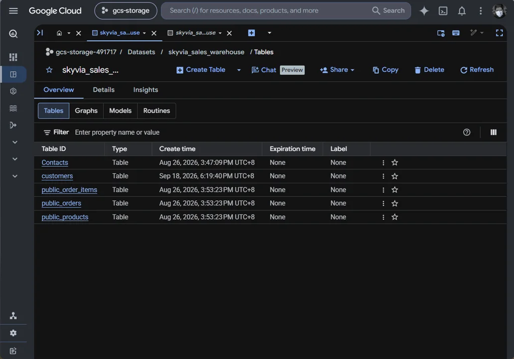
We have the same counterparts in Snowflake and an additional CUSTOMER_CLV table for storing the customer lifetime value (CLV) – a common sales metric.

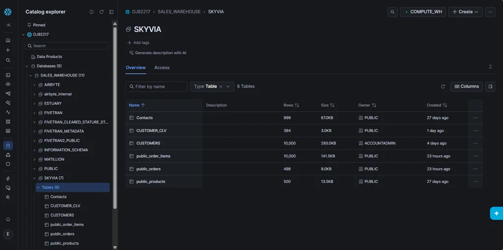
Workload Scope

We are going to move customer and order records, test memory limits, and apply business transformation logic. You will see both Python-made pipelines and Skyvia pipeline examples. Then we will note their runtime durations, rows processed, and evidence that the movement happened in the targets as applicable.

Pipelines in Python will run on a 16GB Linux Mint virtual machine with 6 CPU cores.

Why Is ETL Process Optimization Critical for Modern Data Teams?

ETL process optimization is not just about making a pipeline finish faster. It affects when data becomes usable, how much infrastructure it consumes, and whether downstream systems receive data on time.

Let’s examine some of the reasons.

How Does Pipeline Latency Impact Operational Business Decisions?

It affects data freshness. Consider the following scenarios:

• A pipeline that normally finishes at 7:00 AM but starts taking 90 minutes longer can push dashboards past the time people need them. The dashboard will show yesterday’s data when the sales team starts their morning meeting.
• Delayed warehouse data means executives may be looking at yesterday’s numbers when making decisions today.
• Reverse ETL can propagate stale customer, sales, or support data back into Salesforce, HubSpot, or other operational systems.

Later, you’ll see a test where the entire dataset is processed when only one row changed, while using incremental updates identified the change without reloading the whole thing.

How Do Unoptimized Pipelines Explode Cloud Warehouse Billing?

You will pay for unnecessary compute credits and data scanned. Consider the following scenarios:

• Full refreshes
  If a pipeline reloads 10 million rows when only 10,000 changed, you’re repeatedly processing data that hasn’t changed.
• Inefficient transformations
  Doing a SELECT * FROM large_table followed by transformations you don’t actually need means more data has to be read and processed. And then, repeating this same transformation on a full re-sync means compute usage accumulates.
• Transformation on warehouse compute
  A warehouse transformation can be extremely fast for a small workload, while the cost implications become important as the volume and frequency increase.

The actual billing behavior depends on the warehouse size, workload, concurrency, caching, and billing rules.

What Is the Mathematical Difference Between ETL and ELT Latency?

ETL is Extract from source, Transform, and Load to target. In our test, we extract from PostgreSQL, transform with SQL, and load to Snowflake.

Meanwhile, ELT is Extract raw data from the source, Load it to the target, and Transform. In our ELT example later, we extract the same raw tables in PostgreSQL, load them to Snowflake, and run a SQL transform using Snowflake compute.

These are the conceptual models to move data, not a fixed formula. Some systems overlap these activities or execute them concurrently.

The transformation alone from both ETL and ELT took less than a second in our tests, though the one I ran on Snowflake compute is faster. End-to-end? It’s a different story. Pipeline latency cannot be explained by transformation runtime alone.

What Are the Primary Bottlenecks in the Data Extraction Phase and How Do You Fix Them?

You may experience problems right from the start of your ETL or ELT process. That’s during data extraction. Consider some of them in the following subsections.

Why Should You Switch from Full Table Scans to Incremental CDC?

You want to avoid unnecessary processing. A full load on every pipeline run means deleting all existing data or dropping a table, then recreating the table (if dropped initially) and loading all the extracted data. That captures all the new and updated rows and removes deleted rows all in one shot. But sadly, it includes those that didn’t change at all.

The Problem

While a full table scan is easier to do, using it on very large tables will cause a pipeline to run longer as data volume increases.

The Solution

Extract only the rows that changed. An incremental approach or using Change Data Capture is a preferable choice. If this is not available on your tool of choice, use timestamp watermarking. That is, adding a WHERE clause to your SQL statement, like WHERE modified_date > last_sync_time.

The Full Table vs Incremental Test

We’ll demonstrate them using Skyvia. But the concept applies to any tool you will use.

Below is a pipeline that uses a full table scan and full load:

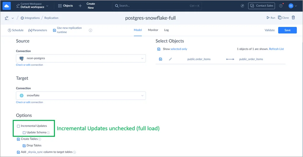
In this test, we will replicate 3603 rows from order_items table from Neon PostgreSQL to Snowflake. Then, we changed 1 row and reprocessed. The above image disables the default incremental updates and forces it to use a full load on every run. Tables in Snowflake are also dropped and created.

Below is the result:

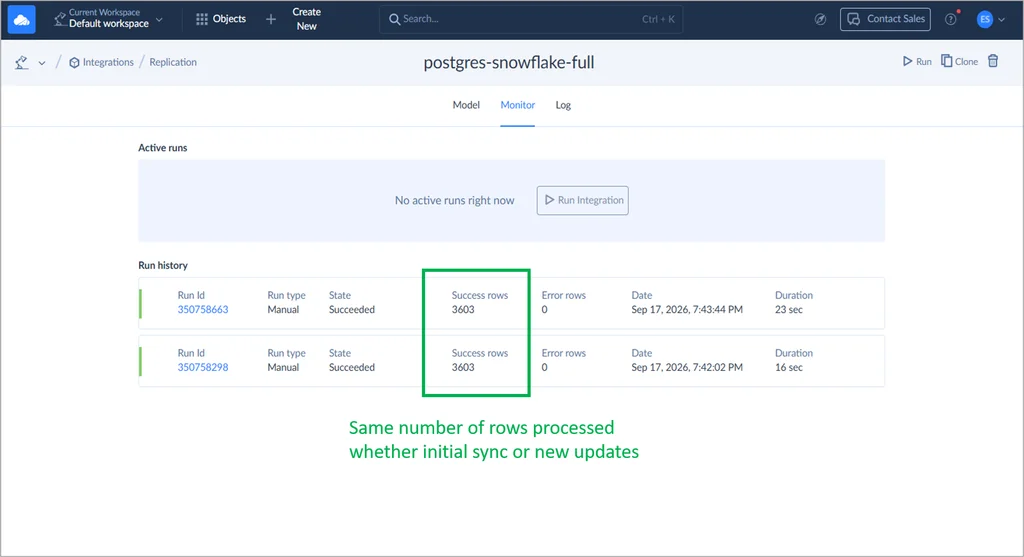
Notice that the same number of rows were processed even though there’s only 1 row that changed. The first run is 16 seconds, and the second run after the row change is 23 seconds.

Below is another pipeline that has the same setup, except the incremental updates are enabled.

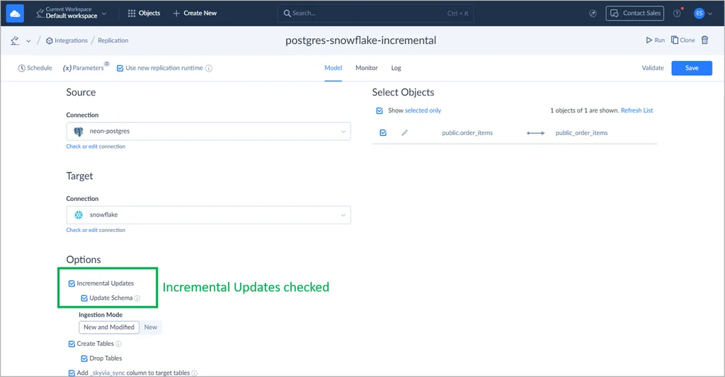
Notice the number of processed rows below. Just 1 for the second run because that’s the only change that happened. The initial run has the same 3603 rows because it did a full load on an empty or missing target.

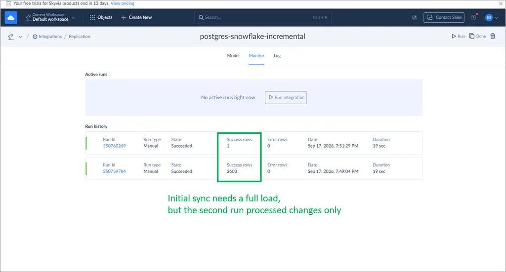
Here’s a comparison of what happened:

Metric	Full Resync	Incremental
Source rows	3603	3603
Rows changed	1	1
Rows extracted	3603	1
Rows loaded	3603	1
Runtime	23 seconds	16 seconds

On a 3.6K-row table, the incremental approach didn’t produce a dramatic runtime improvement because pipeline startup and connection overhead dominated execution time. However, the incremental pipeline transferred only the changed record instead of resynchronizing the entire table.

Doing the incremental approach on a fast-growing table will reveal that extracting only the new and changed rows is better.

How Do You Prevent API Rate Limits and Throttling During SaaS Extraction?

SaaS apps like HubSpot, Salesforce, and Shopify have limits in extracting data using their APIs.

The Problem

Exceeding the API rate limits will trigger an error and compromise data freshness if not fixed soon.

The Solution

Implement backoff retries, dynamic token-bucket rate limiters, and cursor-based pagination. Tools like Skyvia, Fivetran, and others handle these for you. But if your pipeline uses pure coding, you will have to handle these yourself.

Example

Below is a pipeline I made to replicate HubSpot objects to Snowflake. I staged the HubSpot data in DuckDB first before writing the final result in Snowflake.

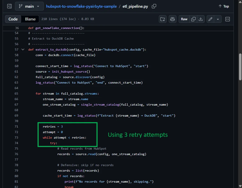
I used retries in case a failure happens. See it below:

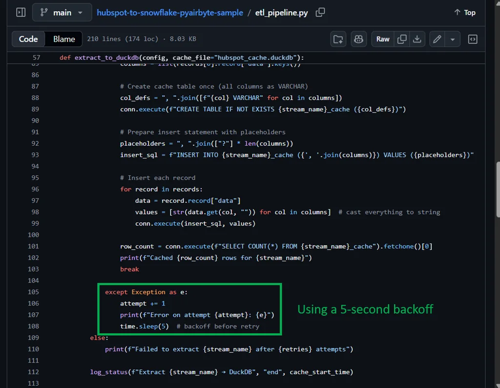
If an error happens, I have to back off for 5 seconds before retrying again. See below:

If you want details about this pipeline, check out my previous article here. You can also find the full code in GitHub.

How Does Database Partitioning Accelerate Source Query Extraction?

Extracting from very large tables can benefit from splitting queries into parallel worker threads instead of loading the whole table in one query.

The Strategy

Use date ranges in the WHERE clause (e.g., WHERE id BETWEEN 1 AND 10000), or use filtered indexes if the database platform supports it. Moreover, use table partitioning. It is supported by major relational database platforms like PostgreSQL, MySQL, and SQL Server.

How Do You Optimize the Data Transformation Phase for Memory Efficiency and Speed?

Transformation shapes the data to its intended format in the target. This section will discuss techniques for doing it effectively.

Why Are Vectorized Transformations Superior to Row-by-Row Loops?

Row-by-row transformation is a sequential approach to examine a row and shape it to its desired format. Meanwhile, there are techniques to transform the rows collectively in a few statements.

The Problem

A row-by-row approach is alright for small datasets. It becomes problematic as your data grows. Your pipeline runs slower as the rows multiply.

The Solution

Depending on your tool, this may be handled collectively. If you use SQL or dbt, it can transform data in sets, not row by row. In Python, you have to handle it through DataFrames for faster results, instead of a row-by-row approach.

Row-by-Row Loops vs. Vectorized Transformation Test

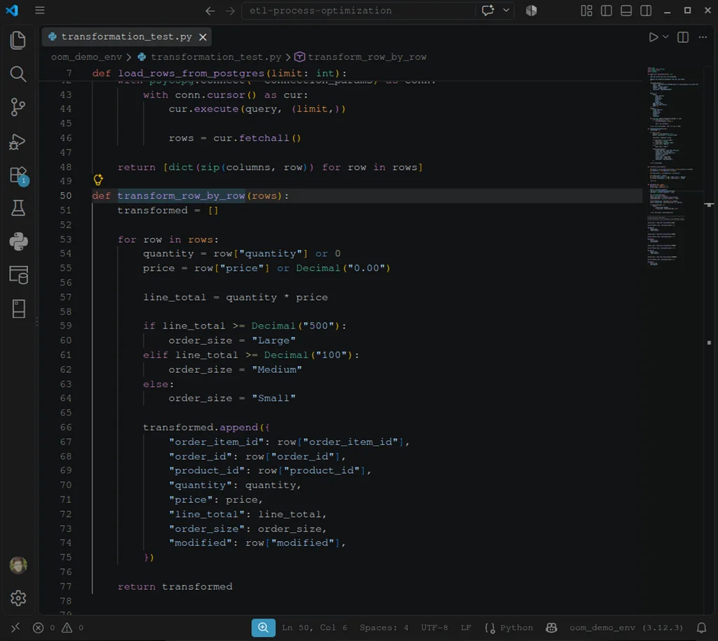
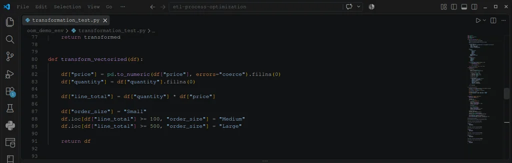
This test involves classifying orders as Small, Medium, or Large, depending on the line total. Line total is computed as price * quantity. If the line total is greater than or equal to 500, it’s large. Medium if it’s greater than or equal to 100. Otherwise, it’s small.

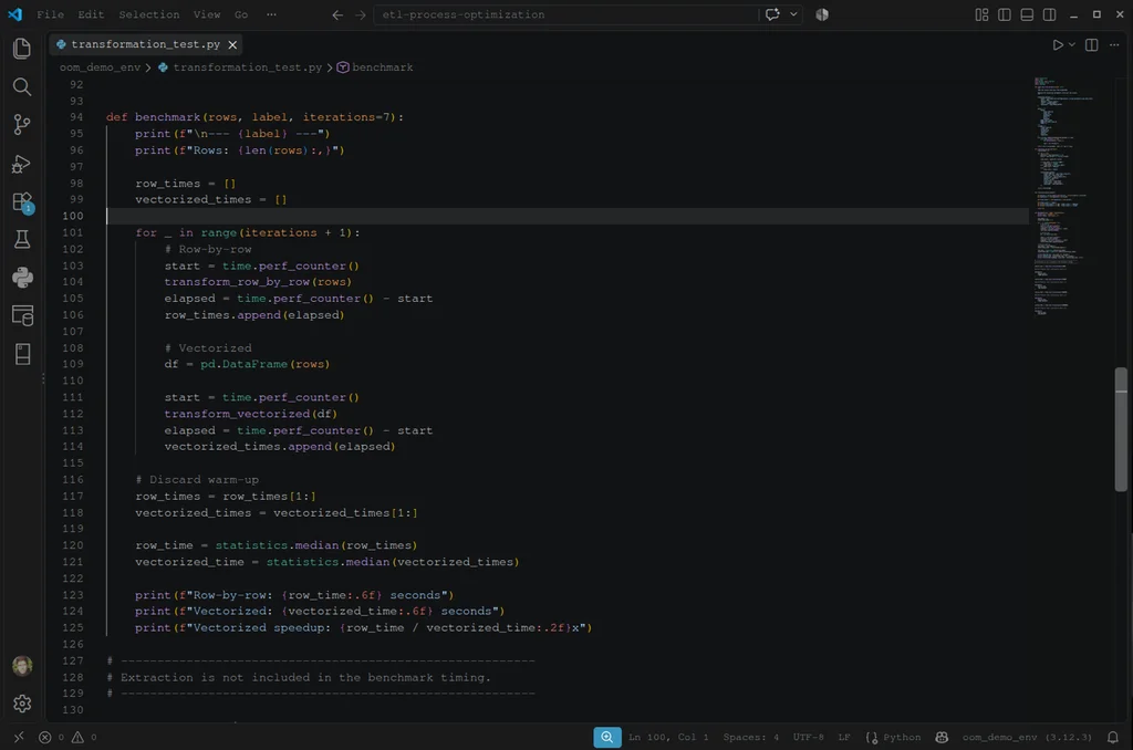
We’re going to use the 1 million order items and compare performance between row-by-row transformation and a vectorized approach using DataFrames. We will measure them based on 1000, 10000, 100000, and 1000000 row sets in a series. Then, we run each set seven times to get the median performance.

First, we need to connect to PostgreSQL and query the order_items table. We pass a limit depending on the size of our rowset.

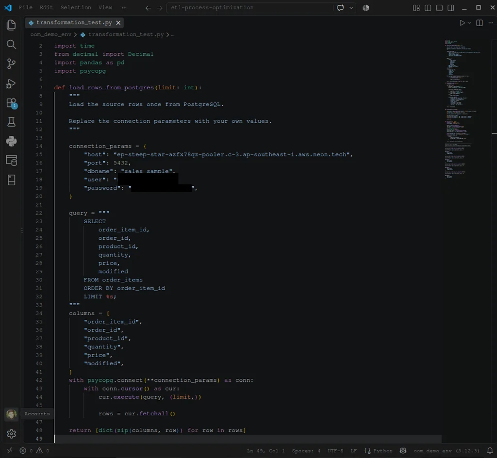
Below is our row-by-row approach using a Python for loop:

Then, we have the shorter DataFrames approach below:

Then, we have our benchmarking function to measure elapsed time 7 times and get the median.

Finally, our orchestration code to divide the process into different rowsets.

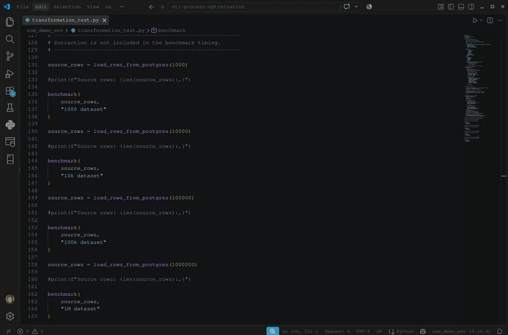
Below is the runtime result. Note that we only measure the elapsed time for transformation because this is a transformation test.

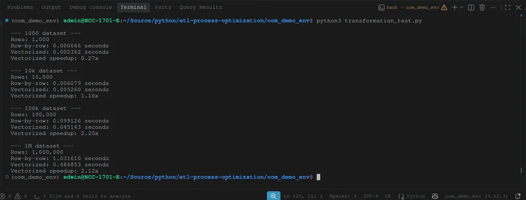
Here’s a summary of the results:

Rows	Row-by-row	Vectorized	Speedup
1,000	0.000646 s	0.002362 s	0.27×
10,000	0.006079 s	0.005260 s	1.16×
100,000	0.099126 s	0.045143 s	2.20×
1,000,000	1.031610 s	0.486853 s	2.12×

The Story Behind the Numbers

• At 1,000 rows, the simple Python loop is much faster. Vectorization takes about 3.7× longer.
• At 10,000 rows, they’re essentially in the same ballpark. Pandas has just started to overcome its overhead.
• At 100,000 rows, vectorization cuts transformation time by more than half: 2.2× faster.
• At 1 million rows, vectorization is about 2.1× faster, reducing the measured transformation from about 1.03 seconds to 0.49 seconds.

In the end, vectorization becomes increasingly useful as the amount of data grows. For small datasets, the overhead of vectorized operations can outweigh their performance benefits.

How Does Pushdown Optimization (ELT) Eliminate Processing Overhead?

Transformation in ELT happens at the warehouse, and warehouse compute can be faster. In the following test, we will compare ETL and ELT transform performance. This is a transformation test also. So, we are not going to measure ETL and ELT pipeline performance end-to-end.

The Strategy

The optimization happens when using warehouse compute for the transformation instead of the compute resources of the source data.

ETL and Pushdown ELT Optimization Example

Our source is a limited 10,000-row order items from 498 orders from our original sources. I used views to limit the result set:

CREATE VIEW vworder_items
AS
SELECT * FROM order_items
ORDER BY order_id, order_item_id
LIMIT 10000;

CREATE VIEW vworders
AS
SELECT * FROM orders
WHERE order_id IN (SELECT order_id from vworder_items);

The transformation involves computing the customer lifetime value.

ETL

The following ETL pipeline involves transforming the data using SQL before reaching Snowflake.

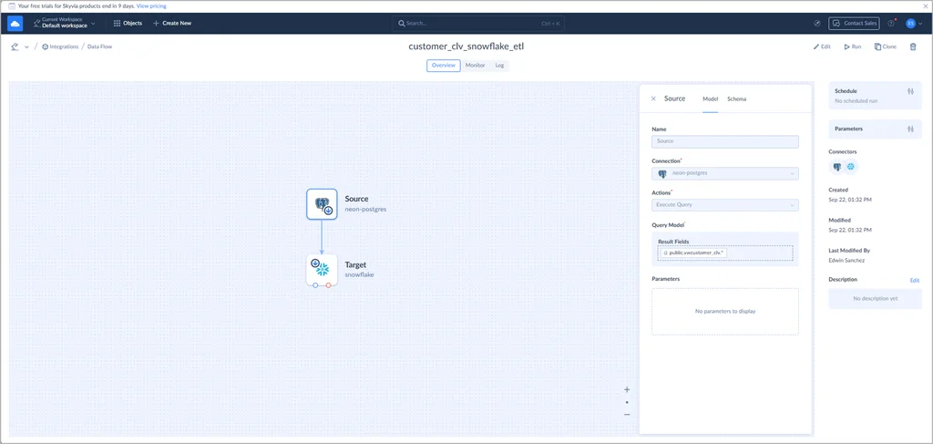
I used another view with the following details:

CREATE VIEW vwcustomer_clv
AS
SELECT 
 o.customer_id 
,SUM(oi.quantity * oi.price) AS lifetime_value
FROM vworders o
inner JOIN vworder_items oi ON o.order_id = oi.order_id
GROUP BY o.customer_id;

Computing per customer will summarize the figures and results to 394 rows. It ran on my test as 9 and 12 seconds, respectively. See below:

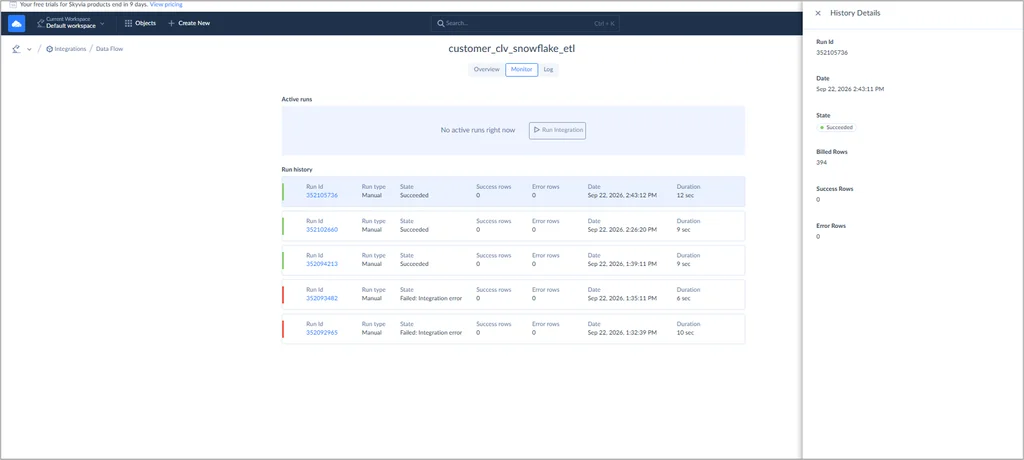
But the 12-second runtime involves the ETL end-to-end runtime duration. Since we can’t see how much time the transformation took, we can get an idea by running the SELECT statement from inside the vwcustomer_clv view. Alternatively, SELECT * FROM vwcustomer_clv will also work.

The query took 625 milliseconds to SUM per customer the price * quantity. See the results in dbForge Studio for PostgreSQL below:

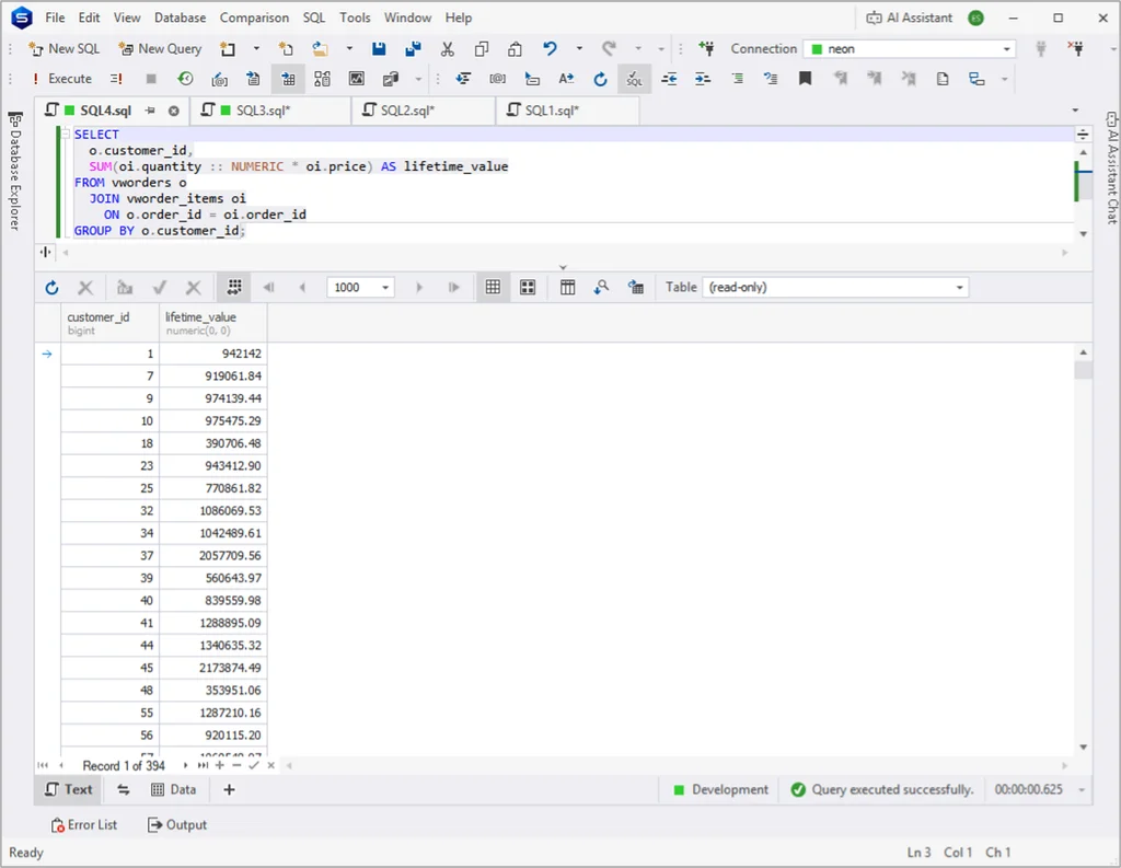
The above helps us a bit to get the SQL transform duration that didn’t appear in the ETL pipeline run.

ELT

Now, let’s try an ELT approach. I started by creating a replication of the raw tables from Neon PostgreSQL to Snowflake. See the setup below:

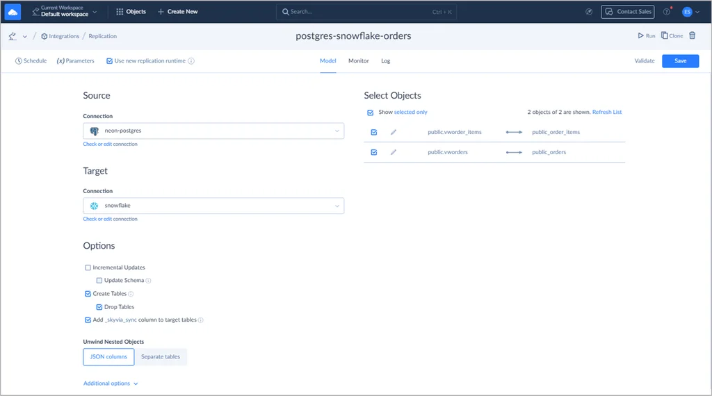
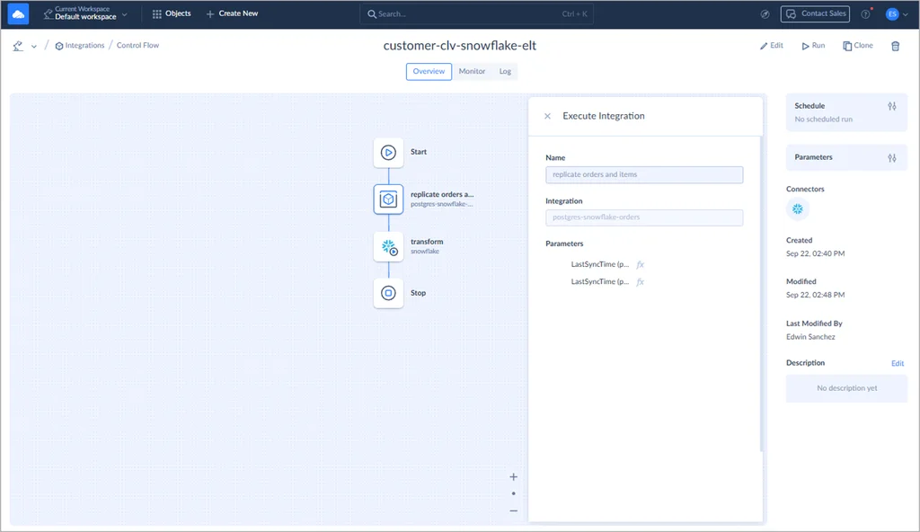
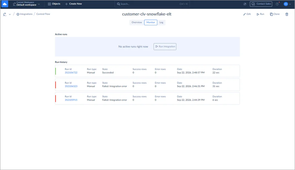
Then, I created a Skyvia Control Flow. Part of the Control Flow is running the replication above. You can see it in the setup below (look for the Integration name). The postgres-snowflake-orders is the first step in the Control Flow:

Then, we did the transformation. The SELECT statement we used is the same as the one used in ETL, with a slight syntax change to adapt to Snowflake SQL. Then, it inserted the results to CUSTOMER_CLV table.

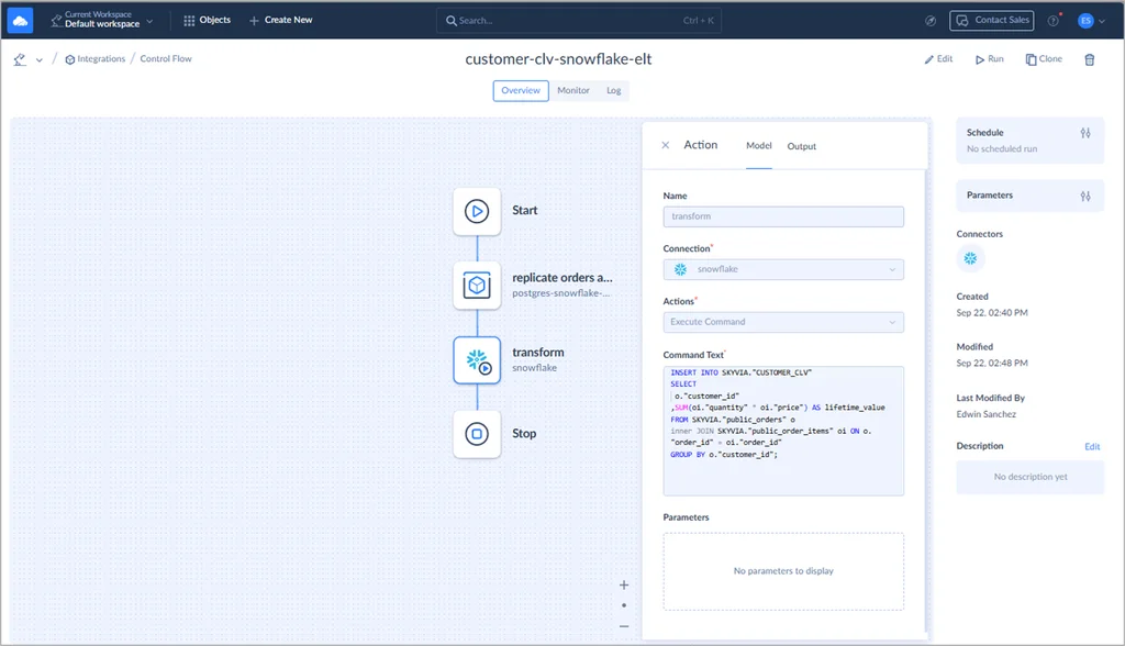
The ELT end-to-end runtime, which involves pushing the raw tables to Snowflake and transforming and storing the transformed results, took 22 seconds.

But we are not measuring the end-to-end runtime duration. We want the transformation duration. Inside Snowflake, the same INSERT..SELECT statement took 409 milliseconds. See it below:

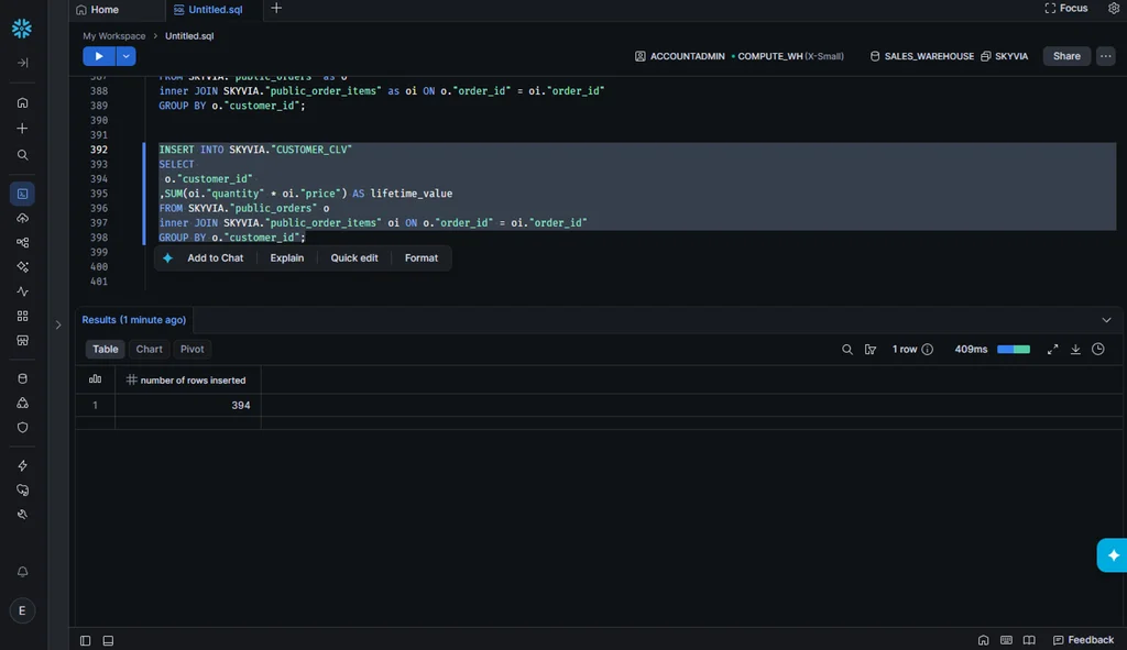
The number of rows transformed is the same as the ETL transformation. The above gives us a slight idea of how long the transform took.

What did this tell us?

Operation	End-to-end Runtime	Transform Runtime	Final Rows in Snowflake
ETL pipeline	12 seconds	~ 625 ms (query from source)	394
ELT pipeline	22 seconds	~ 409 ms (query from Snowflake)	Raw tables replicated: 10,000 order items/ 498 orders Transformed: 394

Using warehouse compute resources in this test proved faster for transformation.

How Do You Prevent Out-Of-Memory (OOM) and Memory Spill Errors?

In SaaS data platforms like Skyvia, Airbyte Cloud, and Fivetran, RAM is managed for you. But it’s a different story in code. You can have out-of-memory errors in code if you don’t manage them effectively. Your Random Access Memory (RAM) can be large today, but not a month or a year later.

The Strategy

Using streaming chunk-parsers for nested JSON/XML data, defining memory bounds per thread, and flushing transformed chunks to temporary disk files before uploading.

A Python Out-of-Memory Example and the Solution to Optimize ETL Process

In this test, we will compare json.load in Python vs ijson. I used a JSON file with 1 million rows, and almost 1 GB in size. Then, I will cap the RAM to 512MB, so the JSON file won’t fit. I used this so my entire laptop won’t crash during this test.

Here’s how to limit the RAM for the Python session in the Visual Studio Code terminal:

ulimit -v 524288   # 512 MB limit

I call the Python code below “bad code” because this will throw a MemoryError:

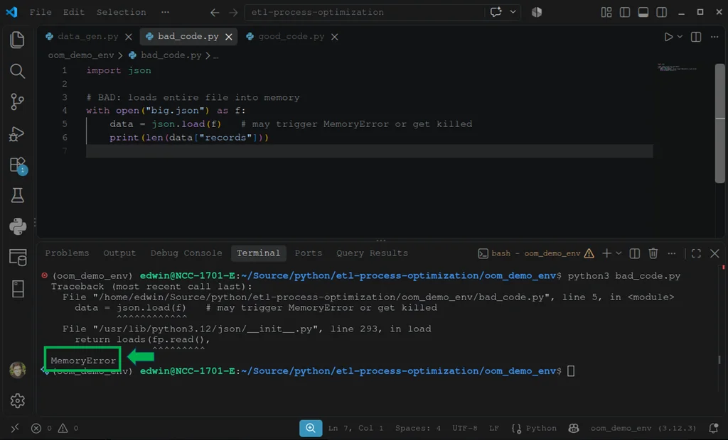
There it is. The json.load can’t read the JSON file at all because of very limited memory.

Meanwhile, the “good code” below will load the big JSON file even with 512MB RAM:

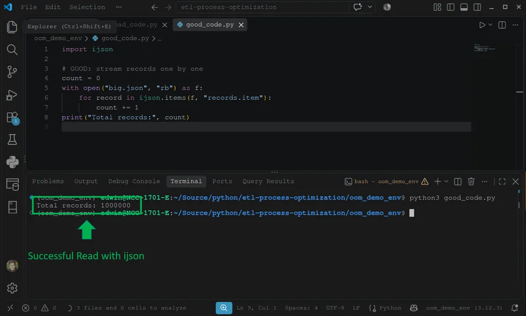
The lesson? Use optimized libraries like ijson to handle processing loads in small chunks.

What Loading Strategies Prevent Database Locks and Accelerate Data Ingestion?

Now, we move to data ingestion. There are also potential problems in this area, as well as ETL process optimization techniques to solve them.

Why Is File Staging with Bulk COPY Commands Faster Than INSERT Statements?

Like the row-by-row example earlier, loops will suffer as the data grows. Even more, INSERT statements will incur massive network round trips and table locking contention.

SaaS data platforms like Skyvia handle the bulk copy for you behind the scenes. So, the next test is applicable to ETL pipelines using code.

The Comparison

I used a Python script to trigger inserts coming from a customer.csv file with 10,000 customers. We will time it and compare it with using Snowflake’s COPY INTO and BigQuery’s bq load. We will assume the CSV file is written and uploaded by a script to a Snowflake STAGE and a Google Cloud Storage bucket.

Row-by-Row Insert vs Snowflake COPY INTO and BigQuery BQ Load

The row-by-row insert is simple: Read the CSV file and insert each row into a BigQuery customer table. Below is the script:

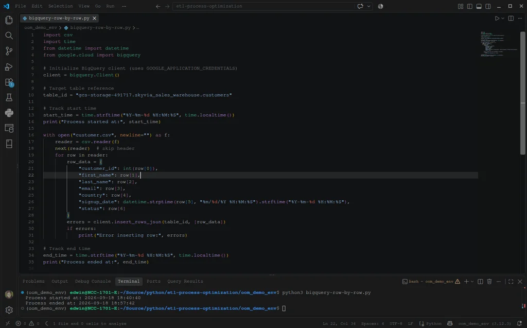
The result is not a surprise. It took more than 17 minutes!

Meanwhile, using the bq load CLI command, the CSV uploads to the table in less than a second. (The zero seconds there is exaggerated. There’s no such thing)

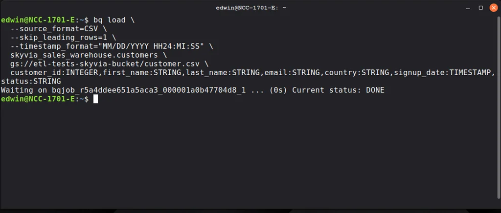
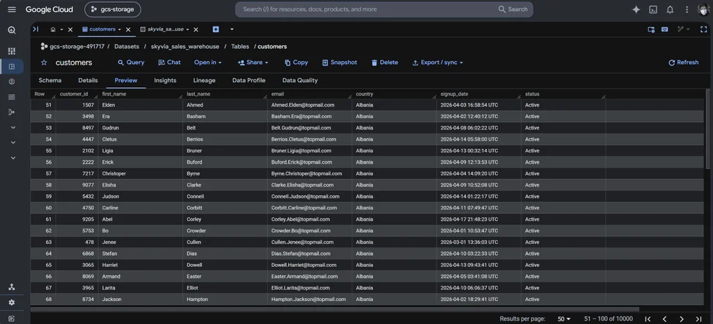
If you preview the customer table in BigQuery, you will see the same 10k rows for both row-by-row inserts and using bq load.

What if we use Snowflake? I copied the CSV file into a Snowflake stage. Then I uploaded the rows using COPY INTO. The upload took 1.2 seconds:

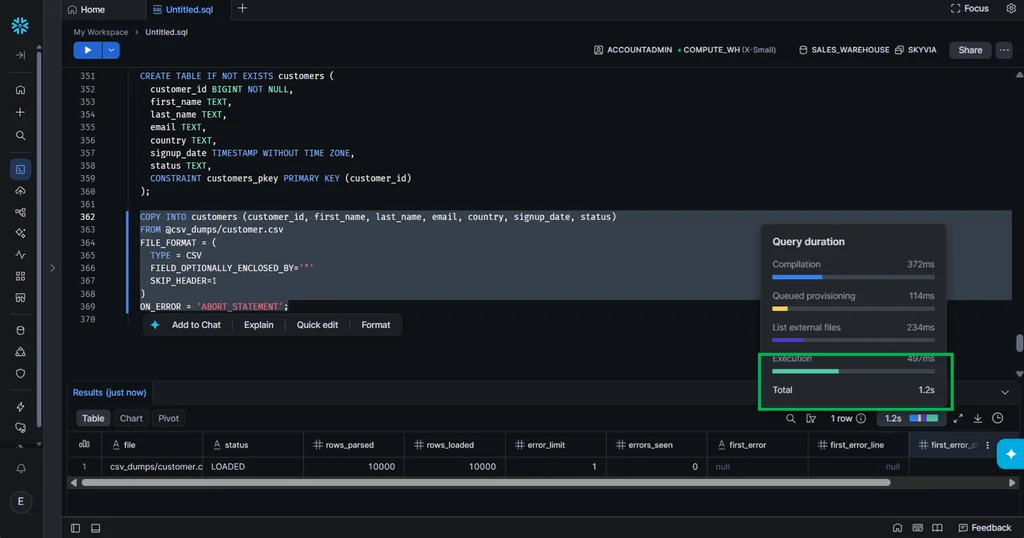
There’s the row count below after the COPY INTO:

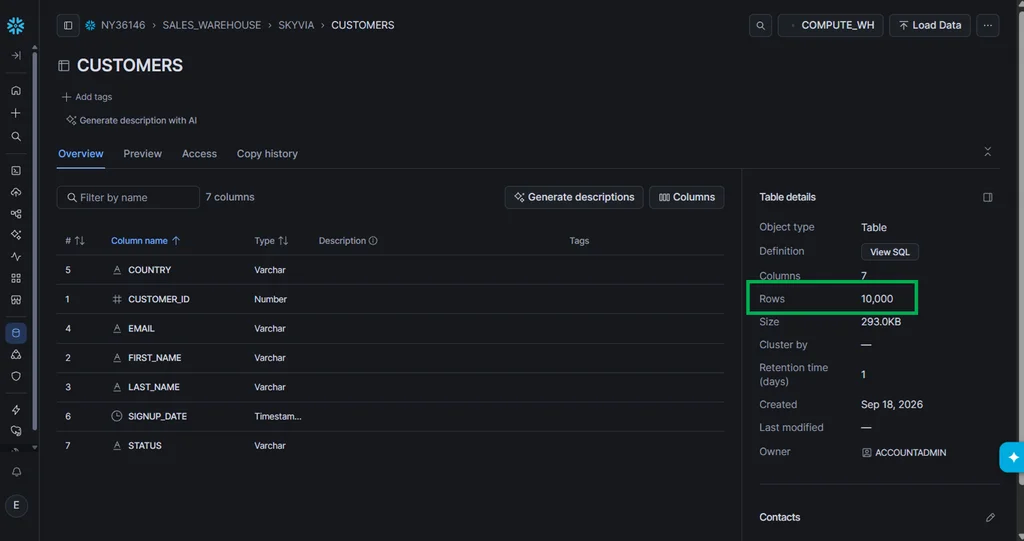
And then, the preview of the table rows:

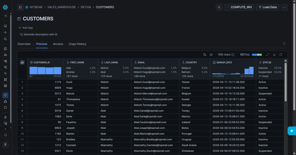
Here’s a summary of the results:

Loading Method	Runtime
Python row-by-row insert	17 minutes 2 seconds
Snowflake COPY INTO	1.2 seconds
BigQuery bq load	less than 1 second

The Python approach took 1,022 seconds, while Snowflake COPY INTO took 1.2 seconds.

That’s roughly 852× faster based on those measurements.

How Do You Balance Real-Time Streaming and Micro-Batch Loading?

It depends on how fresh the data requirement is. Real-time streaming minimizes latency, but more frequent processing can create overhead. Micro-batching groups rows into small batches and reduces processing overhead while keeping data reasonably fresh.

So the question you need to ask is: How stale can the data be before it is considered late?

Consider:

Metric	Streaming	Micro-batching
Latency	Lowest possible	Short Period, up to 1 minute
Data Freshness	Almost immediately, very fresh	Depends on interval
Overhead (API/transaction calls, etc.)	More	Less

Data freshness using a micro-batch instead of real-time streaming can still be considered very fresh depending on your requirement. It also reduces some overhead. Check out the comparison table below:

Batch Window	Approximate Batches / Hour	Data Freshness
1 minute	60	Very fresh
5 minutes	12	Near real-time
15 minutes	4	Slightly delayed
60 minutes	1	Batch-oriented

A 1-minute interval already makes your reports and dashboards new 60 times in an hour. If that is enough for you, you don’t need real-time streaming. But if seconds of delay can piss off hundreds or more customers, then real-time processing is ideal.

The point isn’t that 5 minutes is automatically better than 15 minutes. It’s that the right interval depends on the freshness requirement and the overhead of each batch.

The Strategy

Start with the freshness requirement. If 10–15 minutes is acceptable, micro-batching can eliminate a lot of unnecessary processing overhead.

Some use cases can make this clear:

• Fraud detection -> very few seconds matter a lot
• Operational dashboard -> a few minutes may be acceptable
• Financial or sales reporting -> hourly, daily, weekly, or monthly may be sufficient.

Then, measure the cost of each batch. If you run the process every minute, you pay for the overhead 60 times per hour. But if it’s just 15 minutes, you only pay for it 4 times per hour. That’s the interesting optimization concept.

How Does Proper Indexing and Partition Design Speed Up Target Upserts?

Indexes speed up finding and updating rows, but they also add database overhead when you’re writing large volumes of data. When you do MERGE or upserts, the database engine needs to find existing rows quickly before deciding to update rows or insert new ones. An appropriate index on the match can make that process cheaper to quickly scan the table.

For example:

MERGE INTO customers AS target
USING staging_customers AS source
ON target.customer_id = source.customer_id
...

If customer_id is indexed appropriately, the database engine can locate matching target rows quickly and efficiently.

The Strategy

Load the incoming data into a temporary or staging table first. That is, Source -> Staging table -> MERGE – Target. This is especially useful for remote sources or incompatible data formats. Stage near the target.

Index the match columns. These are the columns needed by the MERGE, like target.customer_id = source.customer_id. Indexing every column will cause more unnecessary write operations. Remember that writing rows also updates the indexes, not just the tables.

For bulk loads, consider disabling or dropping secondary indexes and foreign key constraints to ease the ingestion and make it work faster. Rebuild the indexes and foreign key constraints after the bulk load.

How Do Different ETL Architectural Methodologies Compare Across Key Criteria?

There is no single ETL architecture that minimizes latency, cost, source-system impact, and implementation effort at the same time. You don’t choose one that does everything you need. The right design depends on the workload, freshness requirements, and where you want the processing to occur.

Consider the following criteria, what to measure, and why it matters:

Criterion	What to measure	Why it matters
Extraction latency & source impact	Rows read, query duration, API calls, source CPU	Protects production systems and reduces extraction time
Compute resource consumption	CPU, memory, warehouse runtime	Affects scalability and infrastructure cost
Data freshness SLA	Delay from source change to target availability	Determines whether data is useful for operational decisions
Implementation complexity	Code, orchestration, monitoring, schema handling	Affects development and maintenance effort
Data Volume & Scalability	Processing time, throughput, memory usage, and resource consumption as data volume and change frequency increase	Reveals whether the architecture continues to perform efficiently as workloads grow

What Are the Core Comparison Criteria for Pipeline Architectures?

Let’s expand each of the criteria in the previous table.

Extraction Latency and Source Impact

“How much work does extraction impose on the production system?” – this is the core question for this criterion.

A full table scan might be alright for a small table, but not against a large transactional database. Incremental extraction, timestamp watermarks, and log-based CDC can reduce the amount of data that needs to be read.

Our full vs incremental load testing proves this.

Compute Resource Consumption

Ask yourself:

• Is the ETL server running out of memory?
• Is the warehouse doing expensive transformations?
• Are you transferring huge raw datasets?
• Are you repeatedly consuming warehouse compute?

The json.load() vs. ijson test earlier proves this is very important.

Data Freshness SLA

It’s important to distinguish between pipeline speed and data freshness.

A pipeline that runs every five minutes and takes 30 seconds may provide fresher data than one that completes in 10 seconds but only runs once per hour.

So,

Freshness ≈ scheduling/batching delay + extraction + processing + loading delay

Freshness requirements should drive architectural choices rather than automatically choosing streaming because it sounds faster. These requirements should be in your SLA and be very clear to the team.

Implementation Complexity

This is often overlooked. Even if you use the most technically efficient architecture, you can still find it expensive to maintain if it needs:

• custom CDC logic
• complex orchestration
• schema-change handling
• retry/recovery logic
• monitoring and alerting
• duplicate-event handling
• complicated transformations

In this case, a pipeline under a managed service like Skyvia, even if it consumes more infrastructure resources, might need substantially less custom code or no code at all.

Data Volume and Scalability

The question you need to ask is: “How does the architecture behave as the workload grows?” Because an ETL architecture that performs well with thousands of rows may behave differently when processing millions of rows or more. Scalability measures how performance and resource consumption change as workload size increases.

Measure Performance at Multiple Data Volumes

We did a test earlier on different sets of data: 1K -> 10K -> 100K -> 1M rows. Simulate a test for something like this.

Then compare:

• elapsed time
• rows/second
• memory consumption
• CPU usage
• warehouse compute
• network/data transferred

Data Growth

Then, consider data growth, not just current volume. Because your pipeline might process 100,000 rows today, but might grow to 10,000,000 next year. A row-by-row process became impractical, as proven by our test from 1K to 1M rows. Also, the bulk insert using COPY INTO and bq load proved more than 100x better than inserting row by row.

Change Rate

Consider the change rate too. A table might contain 100 million rows, but only 10,000 changes each day. And another system might contain only a million rows but receives 500,000 changes per hour. Those workloads have very different requirements.

Scalability isn’t simply the ability to process a large dataset once. It is the ability to maintain acceptable performance and resource/compute consumption as data volume and change frequency grow.

Comparison Table: Traditional ETL vs Modern Pushdown ELT vs Real-Time CDC Micro-Batching

We can further compare ETL, ELT, and real-time/micro-batching techniques based on the following metrics:

Architectural Metric	Traditional In-Memory ETL	Modern Pushdown ELT	Real-Time Log CDC Micro-Batching
Primary Execution Location	Intermediate ETL Application Server	Cloud Data Warehouse MPP Engine	Stream Engine + Target Warehouse Staging
Extraction Method	Batch Query / Watermarking	Direct Raw Bulk Transfer	Transaction Log Replication (WAL/Binlog)
Source System Load	Moderate-to-High (Query Overhead)	Low-to-Moderate	Extremely Low (Reads Transaction Logs)
Data Transformation Timing	Pre-Load (In-Flight)	Post-Load (In Warehouse)	Hybrid / Stream Processing
Warehouse Compute Cost Impact	Low Compute, High Network Traffic	High Warehouse Compute Usage	Optimized Micro-Batching Costs
Ideal Data Volume Scale	Small to Medium (<500GB)	Massive / Petabyte Scale	High-Velocity Transactional Data
Memory Spill Vulnerability	High (Requires exact RAM sizing)	Low (Handled by Warehouse Scaling)	Very Low (Stream-driven buffers)

You can match your requirements based on the above information before choosing an approach.

How Can Low-Code Platforms Like Skyvia Simplify ETL Optimization for Non-Engineering Teams?

Low-code platforms like Skyvia simplify ETL process optimization. Instead of handling API rate limits yourself, it does it under the hood. You don’t code column mappings, orchestration, scheduling, and other ETL stuff.

Let’s consider what Skyvia can do that aligns with the tests we did earlier.

How Does Skyvia Implement Pushdown, Automated Watermarking, and Bulk Copy Under the Hood?

We did some of our tests with Skyvia. It wouldn’t be possible without the inherent features needed for ETL process optimization.

Automated Watermark Tracking

Skyvia does it in several ways depending on the integration type used. In the test, I used a Skyvia replication that uses created and modified timestamp columns, like this one:

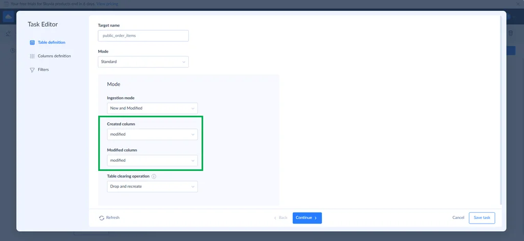
Skyvia will use that to track changes in the source against the target.

Visual Pushdown & In-Flight Transformation Engine

We did an ELT example earlier where we ran an INSERT statement after replicating from PostgreSQL to Snowflake. That statement contains the needed transformation to compute for customer lifetime value, and it ran under Snowflake compute resources. Here’s the pushdown SQL transformation again:

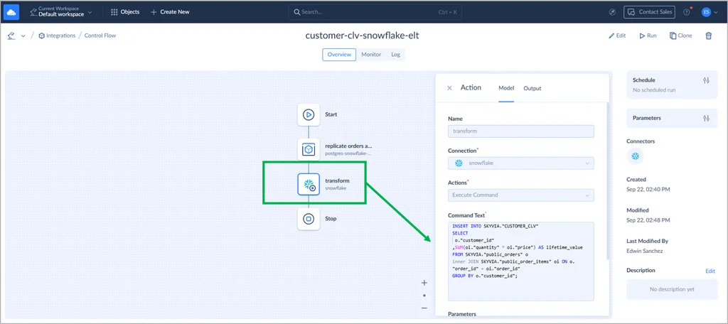
In our ETL example, we used SQL to transform and compute the CLV. But alternatively, it can be done visually using the Expression Builder, like this one:

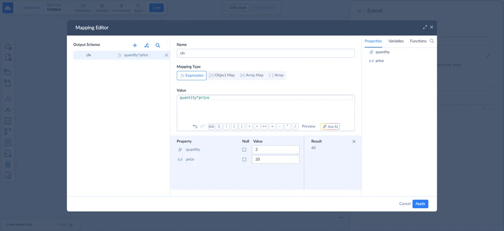
Then, the computed result can be mapped to the appropriate column.

Bulk Copy for Faster Uploads

We used BigQuery as one of our targets. In the BigQuery connection setup, Skyvia has a Cloud Storage Bucket (boxed in green below). This allows Skyvia to stage rows into CSV files and upload it to the specified bucket. That way, Skyvia can do a bulk upload similar to COPY INTO and bq load.

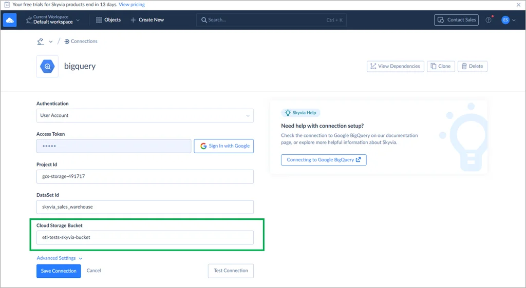
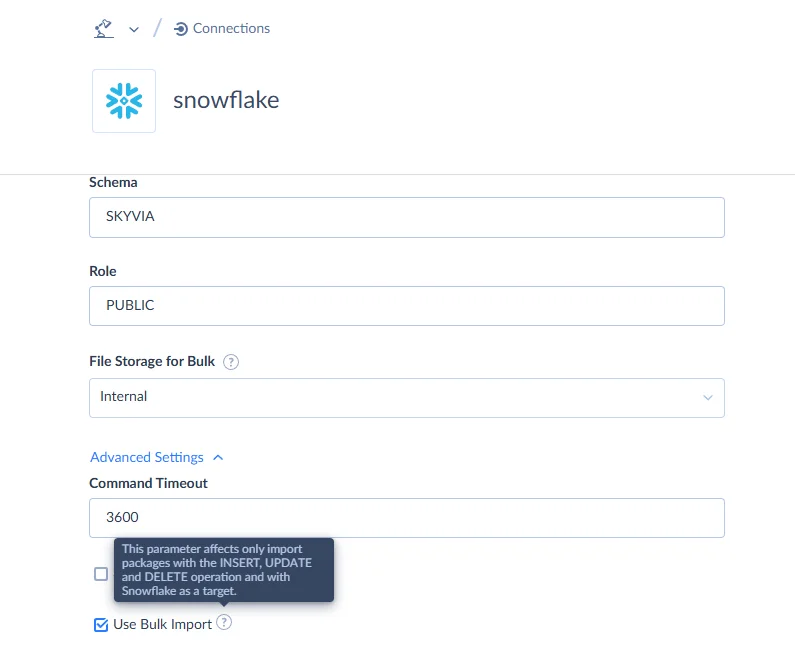
Similarly, the Skyvia Snowflake connection can use a bulk import for a similar approach. See below:

Predictable Non-Usage-Penalty Pricing

Unlike platforms that charge per row ingested, Skyvia uses transparent query/sync packaging, eliminating budget surprises during large database backfills. For this test, I used a Skyvia trial, and below is my consumption based on what I did in the tests:

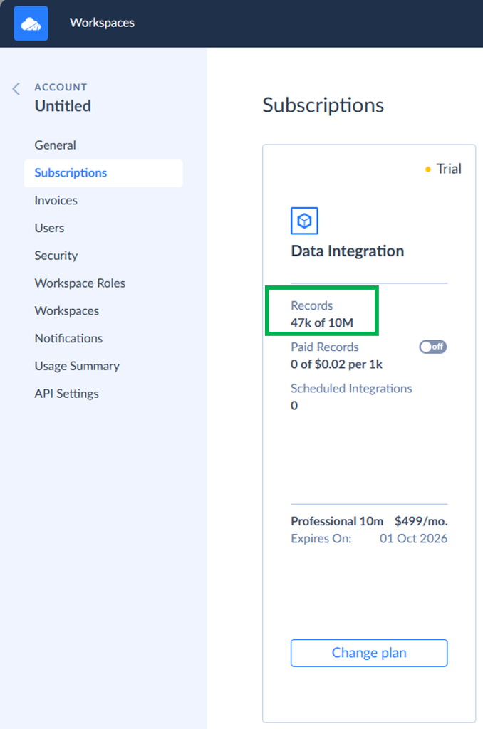
What Are Skyvia’s Honest Technical Limitations?

That said, Skyvia also has limitations like any other tool. Consider some of them below.

Cloud SaaS Only

You can’t install Skyvia on your own infrastructure. It is a 100% cloud-hosted SaaS platform. If your organization operates strict defense, banking, or healthcare workloads that require local air-gapped on-premises deployments with zero outbound cloud egress, Skyvia is not for you.

No Custom Code Compilation

If your transformations require compiling custom Java JARs or Scala scripts directly inside the pipeline runtime, a custom developer-heavy framework (e.g., Apache Spark) is better suited.

What Step-by-Step Blueprint Should You Follow to Optimize Your ETL Pipeline?

Below is the 5-step ETL process optimization.

1: Audit & Profile Current Pipeline Metrics

Earlier, we mentioned comparing runtime duration, CPU/RAM usage, etc. You need to record these metrics to properly profile performance. You don’t just do it during pipeline development, but also while it is running in production to anticipate changes you need to make in the future.

2: Replace Bulk Source Scans with Watermarks or CDC

Optimize early by using incremental load, leveraging CDC or watermarks. Then, follow our scalability tips to choose how to handle workloads.

3: Transition Ingestion to Compressed Staging Files

Some CSV or Parquet files are just too big. You can choose to compress them to GZIP before using bulk commands like COPY INTO for Snowflake.

4: Shift Heavy Transformations to Target Pushdown SQL

Transforming data in our test using pushdown SQL proved faster than transforming before loading. This uses warehouse compute, which is better suited for these transformations. These pushdown SQL should be light enough so as not to consume unnecessary warehouse compute.

5: Set Up Micro-Batch Scheduling and Retry Mechanics

If you’re doing it in code like what we did in some of our tests, establish dynamic retries with backoff strategies to handle temporary API or database network drops gracefully. Also, choose a micro-batching strategy that aligns with your data freshness requirement.

What Are the Key Takeaways for Achieving Long-Term ETL Pipeline Efficiency?

Let’s recap the points that we have proven in our tests:

• Extract: Switch from a full to incremental approach by using watermark tracking or CDC.
• Transform: Move away from row-by-row code loops to vectorized or pushdown SQL.
• Load: Replace row-by-row INSERT by staging to CSV or Parquet files and do a warehouse native bulk copy operation.

ETL process optimization is not a one-time, fire-and-forget thing. It’s an ongoing architectural strategy. Monitor your pipelines and adjust accordingly.

While custom coding with Python and other languages provides the most flexible solution for developer-heavy teams, they demand ongoing pipeline and infrastructure maintenance. It will consume more time. Skyvia simplifies these best practices with automated watermarking, visual pushdown mapping, and bulk loading in a unified platform without maintenance overhead.

Use this 5-step ETL optimization blueprint to develop new pipelines and audit current pipeline infrastructure.

Do you need a managed pipeline that already handles the mentioned complexities? Try out Skyvia for free today.